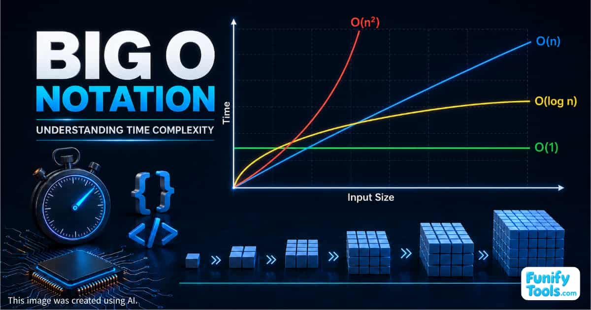
Starting today, I'll also be writing about algorithms and the fundamental ideas behind them.
One concept that appears constantly when discussing algorithm performance is Big O notation.
Big O does not tell us exactly how many seconds an algorithm will take to run. Instead, it describes how the running time or number of operations grows as the input size, usually represented by , becomes larger.
In other words, Big O compares growth rates rather than absolute execution times.
Two algorithms may appear equally fast when the input contains only 100 items. When the input grows to 1,000,000 items, however, one algorithm may still perform well while the other becomes too slow to use in practice.
Big O notation helps us predict and compare those differences.
A Brief History of Big O Notation
Big O notation was not suddenly invented as a method for analyzing computer programs. It developed from asymptotic notation used in mathematics and was later adopted as a standard tool in computer science.
Paul Bachmann
The German mathematician Paul Bachmann is generally credited with introducing the notation.
In an 1894 work, Bachmann used the symbol to represent the “order” or growth rate of a mathematical function.
Edmund Landau
Edmund Landau later helped popularize and formalize the notation. Around 1909, he also introduced little-o notation.
For this reason, Big O and related asymptotic symbols are sometimes called Landau notation or Bachmann–Landau notation.
Donald Knuth
Donald Knuth played an important role in making asymptotic notation a standard part of algorithm analysis in computer science.
Particularly from the 1970s onward, his work helped establish Big O and related concepts such as Theta notation as widely used tools for describing algorithmic complexity.
Why Do We Need Big O Notation?
The same piece of code can take different amounts of time to run depending on many factors, including:
- Processor performance
- Available memory
- Programming language
- Compiler or interpreter optimizations
- Operating system activity
- Implementation details
- Input characteristics
For this reason, comparing algorithms only by measuring execution time is not always fair or useful.
Big O notation allows us to focus on how performance changes as the input grows.
It is useful because:
- Algorithms can be compared by growth rate even when they run on different hardware.
- We can evaluate the general performance of an approach without focusing on every implementation detail.
- It helps predict where bottlenecks will appear as the input becomes larger.
- It makes it easier to decide which parts of an algorithm should be optimized.
How to Calculate Big O Complexity
A practical Big O analysis usually follows these steps:
- Define the input size .
- Count how many times the important operation is performed.
- Express the total amount of work as a function of .
- Keep only the fastest-growing term.
The fastest-growing term determines the final Big O complexity because it eventually dominates the total cost as becomes very large.
Step 1: Define the Input Size
Before calculating complexity, you must decide what represents.
The meaning of depends on the problem:
- For an array or list, is usually the number of elements.
- For a string, is usually the number of characters.
- For a graph, may represent the number of vertices and the number of edges.
- For a matrix, two dimensions such as and may be required.
- For two independent input lists, their sizes may need separate variables.
Defining the input incorrectly can make the entire analysis misleading, so this should always be the first step.
Step 2: Count the Number of Operations
Big O analysis is largely about determining how many times an important operation runs.
The following patterns are enough to analyze many common examples.
A Single Loop Is Usually
If a loop runs times, the operation inside it is also performed times.
for i in range(n):
						    x += 1
The statement x += 1 runs times.
Therefore, the time complexity is:
A Nested Loop Is Usually
If an outer loop runs times and an inner loop also runs times for each outer iteration, the total number of operations is:
for i in range(n):
						    for j in range(n):
						        x += 1
The outer loop runs times, and the inner loop runs times during every outer iteration.
Therefore, the total time complexity is:
A Triangular Nested Loop Can Still Be
The inner loop does not always run exactly times. It may gradually increase with the outer-loop index.
for i in range(n):
						    for j in range(i):
						        x += 1
The number of operations accumulates as follows:
The sum is:
Expanding it gives:
Big O ignores constant factors and lower-order terms, so the result is:
Although the loop performs roughly half as many operations as a full nested loop, both have the same quadratic growth rate.
Repeatedly Halving the Input Is
When the problem size is divided by two during each iteration, the number of iterations grows logarithmically.
while n > 1:
						    n //= 2
The sequence looks like this:
The number of times can be divided by two before reaching 1 is proportional to:
Therefore, the time complexity is:
This pattern frequently appears in binary search, balanced search trees, and algorithms that repeatedly reduce the problem size.
Step 3: Keep the Dominant Term in Sequential Code
When several blocks of code run one after another, their complexities are added.
Suppose a program contains three sections:
- First section:
- Second section:
- Third section:
The total complexity is:
As becomes large, the term grows much faster than the other terms.
Therefore, the overall complexity is:
This does not mean that the other sections take no time. It means that they do not determine the long-term growth rate.
Step 4: Analyze Conditional Branches and Recursion
Conditional Branches
When a program can follow different branches, Big O is commonly expressed using the worst-case branch.
if condition:
						    for i in range(n):
						        pass  # O(n)
						else:
						    for i in range(n):
						        for j in range(n):
						            pass  # O(n^2)
The if branch has a time complexity of .
The else branch has a time complexity of .
Because the worst possible case is quadratic, the overall worst-case complexity is:
If the best-case or average-case complexity is important, it should be analyzed and stated separately.
Recursion
Recursive algorithms can be more difficult to analyze because their repetitions are expressed through function calls rather than visible loops.
The two main questions are:
- How many recursive calls are made at each step?
- How quickly does the size of the problem decrease?
Some common patterns include:
- If each call reduces the problem size by half, the complexity may be .
- If the problem is divided into two halves and combining the results costs , the complexity is often .
- If each call creates two or more additional calls and the recursion tree grows rapidly, the complexity may become or worse.
Merge sort is a classic divide-and-conquer algorithm with a time complexity of:
It divides the input into halves, recursively sorts those halves, and then performs linear work to merge them.
Big O Simplification Rules
Big O notation focuses on long-term growth, so several simplification rules are used.
Ignore Constants
The constant multiplier and constant addition affect actual execution time but not the overall growth category.
Ignore Constant Coefficients
An algorithm that performs operations may be slower than one that performs operations, but both grow linearly.
Keep Only the Highest-Order Term
As becomes large, the quadratic term dominates the linear term.
Ignore the Base of the Logarithm
Logarithms with different constant bases differ only by a constant factor, which Big O notation ignores.
Common Time Complexity Classes
The following table shows how common functions grow as increases. The logarithmic values use base 2.
| Complexity | 1 | 2 | 3 | 4 | 8 | 16 | 32 | 64 | 1,000 |
|---|---|---|---|---|---|---|---|---|---|
| 1 | 1 | 1 | 1 | 1 | 1 | 1 | 1 | 1 | |
| 0 | 1 | 1.58 | 2 | 3 | 4 | 5 | 6 | 9.97 | |
| 1 | 2 | 3 | 4 | 8 | 16 | 32 | 64 | 1,000 | |
| 0 | 2 | 4.75 | 8 | 24 | 64 | 160 | 384 | 9,966 | |
| 1 | 4 | 9 | 16 | 64 | 256 | 1,024 | 4,096 | 1,000,000 | |
| 1 | 8 | 27 | 64 | 512 | 4,096 | 32,768 | 262,144 | 1,000,000,000 | |
| 2 | 4 | 8 | 16 | 256 | 65,536 | 4,294,967,296 | About | About | |
| 1 | 2 | 6 | 24 | 40,320 | 20,922,789,888,000 | About | About | About |
The differences may seem modest when is small, but they become enormous as the input grows.
For example, when :
- requires roughly 10 steps.
- requires roughly 1,000 steps.
- requires roughly 10,000 steps.
- requires 1,000,000 steps.
- requires 1,000,000,000 steps.
- and become effectively impossible for most practical purposes.
Common Big O Complexity Categories
: Constant Time
The amount of work remains roughly the same regardless of the input size.
value = numbers[0]
Accessing an array element by index is generally a constant-time operation.
: Logarithmic Time
The search space is repeatedly reduced, often by half.
Binary search is the most familiar example.
: Linear Time
The algorithm performs work proportional to the number of input elements.
Scanning every item in a list is a typical linear-time operation.
: Linearithmic Time
Many efficient comparison-based sorting algorithms fall into this category.
Examples include merge sort, heap sort, and the average-case performance of quicksort.
: Quadratic Time
Quadratic complexity commonly appears in nested loops that compare many pairs of input elements.
Simple sorting algorithms such as bubble sort, selection sort, and insertion sort have worst-case behavior.
: Cubic Time
Cubic complexity often appears in algorithms with three nested loops, such as some basic matrix-processing methods.
: Exponential Time
Exponential algorithms often explore every possible combination through branching recursion.
A naive recursive implementation of Fibonacci numbers is a common introductory example.
: Factorial Time
Factorial complexity appears when an algorithm examines every possible ordering of elements.
Brute-force solutions to some permutation and traveling-salesperson problems can have this type of growth.
Big O Does Not Predict Exact Running Time
Big O is not a stopwatch.
It does not tell us precisely how long an algorithm will run on a particular computer. It describes how the required work grows as the input size increases.
An algorithm can sometimes be slower than an algorithm for small inputs because of constant factors, memory access patterns, setup costs, implementation quality, or hardware characteristics.
For example:
may be greater than:
when is small enough.
However, as continues to grow, the quadratic function eventually overtakes the linear one and then grows much faster.
Big O is most valuable when we want to understand scalability rather than benchmark a single run.
Why Big O Matters in Real Software
During the early stages of development, datasets are often small. Almost any implementation may appear fast enough.
As a service grows and data accumulates, however, small inefficiencies can expand rapidly.
A section of code that originally seemed harmless—perhaps “just one more loop”—can eventually become a bottleneck that increases response times, raises server costs, and damages the user experience.
Big O analysis helps developers identify these risks before they become serious production problems.
It also prevents optimization from becoming a matter of guesswork.
Instead of looking at code and saying, “This part feels slow,” developers can examine which operation dominates as the input grows.
In many situations, slightly improving an operation provides far less benefit than redesigning an algorithm so that it becomes or .
Understanding Big O therefore makes it easier to prioritize optimization work and decide where engineering effort will have the greatest effect.
Big O and Practical Performance Are Both Important
Big O is extremely useful, but it does not describe every aspect of performance.
Two algorithms with the same time complexity can behave very differently in real applications because of:
- Constant factors
- Memory usage
- Cache efficiency
- Input distribution
- Network or disk access
- Parallel processing
- Language overhead
- Database behavior
- Compiler optimization
For example, two algorithms may both be , but one may scan the data once while the other scans it ten times. They belong to the same growth category, but the first is likely to be faster in practice.
Big O should therefore be combined with real benchmarks, profiling, and knowledge of the expected input.
It tells us how an algorithm scales. Measurement tells us how it actually performs in a particular environment.
Space Complexity Also Matters
Although Big O is frequently used to describe running time, it can also describe memory usage.
An algorithm may run quickly but require a large amount of additional memory. Another algorithm may use very little memory but take longer.
For example:
- An algorithm using only a few variables may require extra space.
- Copying all input elements may require extra space.
- Building a two-dimensional table may require space.
In real systems, developers often have to balance time complexity and space complexity rather than optimizing only one of them.
How to Get Better at Big O Analysis
When learning Big O, there is no need to memorize every formula immediately.
A better approach is to develop an intuitive understanding of how loops, recursion, algorithms, and data structures affect performance.
Start by asking a few simple questions:
- How many times does this code repeat?
- Are the loops nested or sequential?
- Does the problem size decrease during each step?
- Does the algorithm divide the input into smaller parts?
- Does it perform an expensive operation such as sorting or searching?
- Are there multiple independent input sizes?
- Which part grows fastest as the input becomes larger?
- How much additional memory does the algorithm use?
Once these questions become habitual, even complicated code becomes easier to analyze.
Final Thoughts
Big O notation is not a tool for predicting exact execution time. It is a way to compare how algorithm performance changes as the input grows.
Once you become familiar with this perspective, you can identify sections of code that may become problematic at scale much more quickly.
Ultimately, Big O is not simply about making software faster today. It is about designing software that will not collapse as its workload grows.
Almost any code can appear fast when the input is small. Building a system that continues to perform reliably with larger datasets is a very different challenge.
Big O gives developers a framework for understanding that difference.
In the next article, we will examine several major algorithms and see how these ideas apply to real examples.
Thank you for reading, and I hope you have a wonderful day!
This article is also available in Korean: Read the Korean version