What the calculator shows
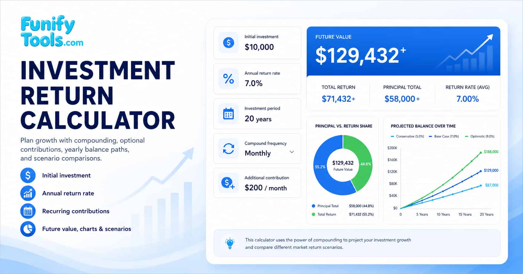
The Investment Return Calculator projects how a lump sum or recurring investment may grow over a chosen time horizon using compound interest. It combines your starting balance, any recurring contributions, and the projected return or loss generated over the selected period. The result page displays the total future value, total return or loss, investment value breakdown, a donut chart, a yearly bar chart, and a year-by-year balance table. It also provides a scenario comparison feature so you can test multiple assumptions side by side before saving the result to Funify Notes for later reference.
Whether you are planning for retirement, saving for a child's education, or evaluating a potential investment portfolio, this calculator helps you visualize how different inputs affect long-term outcomes. The summary focuses on total future value and total return, while the chart, step-by-step output, percentage bars, and yearly table make it easier to see how the final amount is built over time. To see how professional financial planners approach similar projections, you can search Google for investment growth projection best practices and compare the methodology used by industry experts.
Compounding basics
Compounding is the process where returns are reinvested and begin generating their own return, creating exponential growth over time. When compounding happens more often, for example monthly instead of yearly, the ending value is usually slightly higher because gains are added back into the balance sooner. This effect becomes more pronounced over longer time horizons and higher return rates.
Understanding compounding is essential for long-term financial planning. Even a modest annual return, when compounded consistently over decades, can turn a small initial investment into a substantial nest egg. The key variables that determine the power of compounding are the initial principal, the annual rate of return, the compounding frequency, and the total time the money is allowed to grow. The table below illustrates how different compounding frequencies affect a $10,000 investment at a 7% annual return over 20 years.
| Compounding frequency | Ending balance | Total return | Difference vs. yearly |
|---|---|---|---|
| Yearly | $38,696.84 | $28,696.84 | Baseline |
| Semi-annual | $39,592.60 | $29,592.60 | +$895.75 |
| Quarterly | $40,063.92 | $30,063.92 | +$1,367.07 |
| Monthly | $40,387.39 | $30,387.39 | +$1,690.54 |
| Daily | $40,546.56 | $30,546.56 | +$1,849.71 |
FV = P x (1 + r / n)^(n x t)
Initial investment + recurring contributions
Future value - principal total
In the basic formula, P is the initial investment, r is the annual return rate expressed as a decimal, n is the number of compounding periods per year, and t is the number of years. Recurring deposits are added according to the selected contribution schedule in the calculator logic. For a deeper dive into the mathematics, you can search Google for compound interest future value formula and compare the worked examples with the values shown by this page.
Investment types and typical use cases
Different asset classes carry different risk and return characteristics. Stocks (equities) are often chosen for long-term growth and capital appreciation, though they come with higher volatility. Bonds (fixed income) are used for income generation and portfolio stability, typically offering lower but more predictable returns. Real estate may provide rental income and property appreciation over time. Diversified funds such as index funds, exchange-traded funds (ETFs), and target-date funds can reduce single-asset risk by spreading investments across multiple securities and sectors.
The expected annual return you enter into the calculator should match the asset mix, fees, taxes, and time horizon you are modeling. For example, a conservative portfolio weighted toward bonds might use a 3-5% expected return, while a growth-oriented stock portfolio might use 7-10%. For historical context, you can search Google for historical stock bond portfolio returns and use conservative, base, and optimistic cases instead of relying on a single number.
What affects return the most
Three inputs matter most in long-range planning. First, the annual return rate changes the slope of the growth curve - a difference of just 1% can compound into a significantly different ending balance over 20 or 30 years. Second, the time period gives compounding more time to work; the longer the horizon, the more dramatic the exponential effect. Third, recurring contributions can materially increase the final value even when the return rate stays the same, because they add new principal that itself begins to earn returns.
| Input | Main effect | What to test |
|---|---|---|
| Annual return rate | Changes the growth curve and total return. | Compare conservative, base, and optimistic rates. |
| Investment period | Gives compounding more or less time. | Compare short, medium, and long time horizons. |
| Recurring contribution | Raises principal and can become a major part of future value. | Test monthly and yearly deposit amounts. |
| Compounding frequency | Changes how often gains are added back to the balance. | Compare yearly and monthly compounding. |
Practical examples by investment goal
The table below illustrates how the same calculator can be used for different financial goals. Each scenario uses a distinct combination of initial investment, contribution pattern, time horizon, and expected return to show the range of possible outcomes.
| Goal | Initial investment | Monthly contribution | Time horizon | Expected return | Est. future value |
|---|---|---|---|---|---|
| Emergency fund | $5,000 | $200 | 3 years | 3% | $12,800+ |
| College savings | $10,000 | $300 | 10 years | 6% | $67,000+ |
| Retirement (early) | $25,000 | $500 | 20 years | 7% | $360,000+ |
| Wealth building | $50,000 | $1,000 | 30 years | 8% | $1,500,000+ |
These figures are illustrative only. Actual results will vary based on market conditions, fees, taxes, and the specific investments chosen. Use the scenario comparison feature in the calculator to customize these examples with your own numbers.
Using scenarios
Use the scenario comparison table to test different deposit sizes, rates, periods, and compounding choices instead of relying on a single projection. A small change in return assumption can compound into a large difference over long periods, while a higher contribution can make results less dependent on the return rate alone. This is especially useful when you are uncertain about future market conditions and want to see a range of possible outcomes.
A practical workflow is to calculate a conservative case first, add it as a scenario, then raise the contribution or time period and compare the ending balance. You can also test what happens if the annual return is lower than expected, or if you increase your monthly deposits mid-way through the investment period. This makes the result more useful for savings goals, retirement planning, education funding, and long-term portfolio reviews.
Compounding frequency comparison
Choosing between yearly and monthly compounding is one of the settings available in this calculator. The difference may seem small on a single year, but over extended periods the more frequent compounding schedule can add thousands of dollars to the final balance. The table below compares yearly and monthly compounding across different investment horizons for a $10,000 initial investment with a 7% annual return and no additional contributions.
| Time horizon | Yearly compounding | Monthly compounding | Difference |
|---|---|---|---|
| 5 years | $14,025.52 | $14,176.25 | $150.73 |
| 10 years | $19,671.51 | $20,096.61 | $425.10 |
| 15 years | $27,590.32 | $28,489.47 | $899.15 |
| 20 years | $38,696.84 | $40,387.39 | $1,690.54 |
| 30 years | $76,122.55 | $81,164.97 | $5,042.42 |
As the table shows, the advantage of monthly compounding grows with time. For a 30-year investment, monthly compounding adds more than $5,000 compared to yearly compounding on the same initial principal. When recurring contributions are added, the gap becomes even larger because each deposit benefits from more frequent compounding as well.
Risk and return trade-off
Every investment involves a trade-off between risk and potential return. Higher expected returns typically come with higher volatility and a greater chance of short-term losses. Lower-risk investments such as government bonds or high-yield savings accounts offer more stability but generate lower long-term growth. Understanding this relationship is critical when choosing the annual return rate to enter into the calculator.
The table below summarizes common asset classes and their historical risk-return profiles to help you choose realistic input values for your projection.
| Asset class | Typical annual return range | Volatility level | Best for |
|---|---|---|---|
| Cash & money market | 1% - 3% | Very low | Short-term savings, emergency reserves |
| Government bonds | 2% - 5% | Low | Income, portfolio stability, capital preservation |
| Corporate bonds | 3% - 6% | Moderate | Higher income, moderate growth with some risk |
| Diversified stock portfolio | 6% - 10% | High | Long-term growth, retirement, wealth building |
| Real estate (REITs) | 4% - 12% | Moderate to high | Income plus appreciation, inflation hedge |
| Small-cap / emerging markets | 8% - 15% | Very high | Aggressive growth, high risk tolerance |
When using this calculator, choose an annual return rate that reflects your actual asset allocation and risk tolerance. For a balanced portfolio of 60% stocks and 40% bonds, a 5-7% expected return is common. For an aggressive all-stock portfolio, 7-10% may be appropriate. Always test multiple scenarios with different rates to understand how sensitive your plan is to the return assumption.
Assumptions and what is not included
- The annual return rate is assumed to be steady during the projection period. Real markets fluctuate year to year.
- Recurring contributions are added at the end of the selected contribution period (monthly or yearly).
- The calculator does not include taxes, trading fees, advisory fees, fund expense ratios, currency exchange effects, or inflation.
- Actual investment results can be higher or lower than the projection due to market volatility and economic conditions.
- The projection assumes all returns are reinvested and no withdrawals are made during the investment period.
To adjust the estimate for purchasing power erosion, you can search Google for inflation adjusted investment return calculator and compare nominal growth with real (inflation-adjusted) values.
References
Investment overview | Compound interest basics | Future value